Transition-state analysis

Use this workflow for frequency outputs that contain a transition-state candidate. MolOP can select candidate frames, inspect imaginary modes, and generate geometry-based endpoint candidates. It does not optimize those structures or certify a reaction path.

Select candidate frames

Python

from molop import AutoParser

batch = AutoParser("results/*.log")
normal = batch.filter_state("normal", n_jobs=-1)
ts_batch = normal.filter_state("ts", n_jobs=-1)

print("parsed:", len(batch))
print("normal:", len(normal))
print("transition-state files:", len(ts_batch))

Selection result (input-dependent)

Text Only

parsed: <count>
normal: <count>
transition-state files: <count>

The counts depend on the input directory. A file can contain several frames, so select the actual TS frame rather than assuming that parsed_file[-1] is the one selected by filter_state("ts"):

Python

for parsed_file in ts_batch:
    for frame in parsed_file:
        if frame.is_TS:
            imaginary = frame.vibrations.num_imaginary if frame.vibrations else None
            print(parsed_file.filename, frame.frame_id, imaginary)

Candidate-frame output shape (input-dependent)

Text Only

<source filename> <frame_id> <imaginary-mode count or None>

is_TS is a programmatic candidate decision. None means that the source did not provide enough evidence and is different from False.

Inspect the imaginary mode

Python

ts_frame = next(
    (frame for parsed_file in ts_batch for frame in parsed_file if frame.is_TS),
    None,
)
if ts_frame is None:
    raise ValueError("No transition-state frame was found in the input")
vibrations = ts_frame.vibrations

if vibrations is None:
    raise ValueError("The TS candidate has no structured frequency data")

print("imaginary modes:", vibrations.num_imaginary)
print("frequencies (cm^-1):", vibrations.frequencies.m_as("cm^-1"))

Imaginary-mode output (input-dependent)

Text Only

imaginary modes: <count>
frequencies (cm^-1): <frequency array>

Review the frequency sign, displacement direction, and chemical interpretation. The number of imaginary modes alone is not a reaction-path validation.

Generate structures along the mode

ts_vibration displaces coordinates along the unique imaginary mode and returns candidate Molecule objects. It requires frame.is_TS to be true and may omit geometries that violate basic crowding checks:

Python

candidates = ts_frame.ts_vibration(ratio=1.75, steps=7)
print("candidate geometries:", len(candidates))

Imaginary-mode candidates (image output)

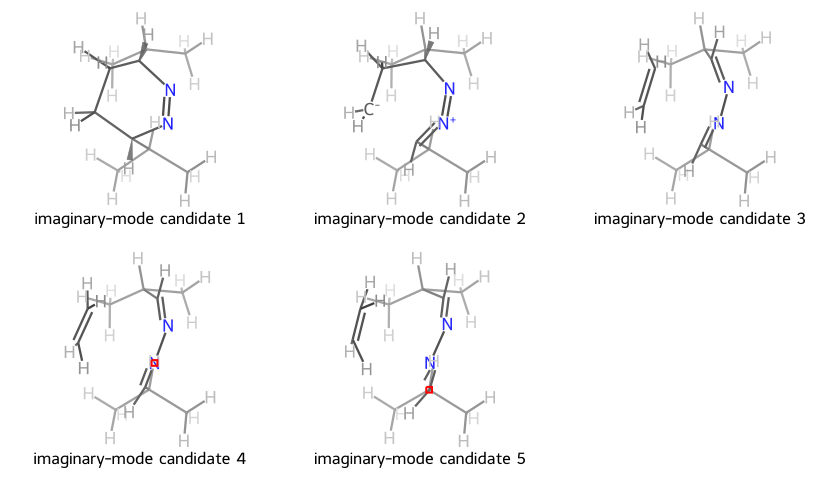
The image is generated from a real parsed frame with one imaginary mode. Each panel is a ts_vibration(...) candidate for which graph reconstruction succeeded. The two-dimensional layout compares connectivity; it is not an optimized reaction path.

Render animations

Use draw_animation(...) on any parsed file to render its valid frames as a GIF or animated SVG. This covers optimization, IRC, and scan trajectories. Frames that cannot reconstruct an RDKit graph are skipped; rendering fails only when no frame is drawable. The default legend retains the original frame ID, adds TS for transition-state frames, and includes total energy when available.

Python

trajectory = ts_batch[0]
trajectory.draw_animation(file_path="trajectory.gif", duration=120, size=(640, 480))
trajectory.draw_animation(
    image_format="svg",
    file_path="trajectory.svg",
    duration=120,
    size=(640, 480),
)

For a selected normal mode, use draw_vibration_animation(...); the TS-specific method selects the unique imaginary mode automatically. Their default legends include the mode index, frequency, and candidate position. Pass legends=[...] to either method to supply labels explicitly.

Python

ts_frame.draw_vibration_animation(vibration_id=0, file_path="mode-0.gif", steps=9)
ts_frame.draw_ts_vibration_animation(file_path="ts-imaginary-mode.gif", steps=9)

Infer endpoint candidates and bond changes

Python

try:
    mapped_rxn = ts_frame.to_mapped_rxn_smiles()
    print(mapped_rxn)
except ValueError as exc:
    print("endpoint inference failed:", exc)

difference = ts_frame.to_diff_rdmol()
if difference is not None:
    print("difference graph bonds:", difference.GetNumBonds())

to_reaction obtains its endpoints from possible_pre_post_ts, assigns each atom the 1-based map number from its source atom order, and returns an RDKit ChemicalReaction. to_mapped_rxn_smiles() uses that frame-level reaction directly and exports non-canonical reactants>>products RXN SMILES. To request additional endpoint sampling, call ts_frame.to_mapped_rxn_smiles(additional=True).

Endpoint candidates and virtual-bond difference (image output)

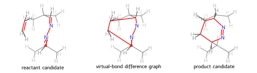
Red highlights identify bonds that change between the endpoint candidates. The center panel comes from to_diff_rdmol(). Its zero-order bonds are MolOP’s machine-readable difference markers; the generator promotes them to visible lines only in the drawing copy.

possible_pre_post_ts returns geometry-based endpoint candidates, not optimized reactant and product structures. to_diff_rdmol can return None when no supported bond-breaking difference is inferred. Review atom mapping, connectivity, and the original calculation before using either result in an automated reaction workflow.

By default, endpoint inference samples eight amplitudes on each side of the imaginary mode from min_ratio=0.6 to max_ratio=1.4, evenly spaced in harmonic-oscillator potential energy. It votes for the most frequent reconstructed topology separately in the negative and positive displacement spaces, retaining the largest-amplitude conformer for the winning topology. The candidate with more disconnected fragments is returned as the precursor; equal fragment counts preserve negative-side then positive-side order. Use steps to change the number of amplitudes sampled on each side.

The default sampling_method is "harmonic_potential". To retain the original linear-amplitude sampling, set sampling_method="amplitude" explicitly:

Python

reactant, product = ts_frame.possible_pre_post_ts(
    show_3D=True,
    sampling_method="amplitude",
)

The harmonic-potential method uses a_i = sqrt(a_min**2 + i * (a_max**2 - a_min**2) / (steps - 1)), which spaces a**2 and therefore the harmonic potential evenly. For an imaginary mode, this corresponds to evenly spacing the magnitude of the potential-energy decrease away from the saddle. The "amplitude" method preserves the original linear-amplitude sampling. The default "harmonic_potential" method spaces potential energy evenly, while "amplitude" preserves the original linear-amplitude behavior. The same option is available on additional_pre_post_ts, save_pre_post_ts, and to_diff_rdmol.

The standard endpoint pair remains the primary result. For an additional representation, retain the endpoint conformers and resample the atoms not incident to changed bonds while fixing the changed atoms at their endpoint coordinates:

Python

standard_pre, standard_post = ts_frame.possible_pre_post_ts(show_3D=True)
additional_pre, additional_post = ts_frame.additional_pre_post_ts(standard_pre, standard_post)

When no bonds change between the standard endpoints, the additional sampling returns that same pair.

The following Notebook image compares the standard and additional-sampling results on a real TS frame. Because the additional sampling fixes only atoms incident to changed bonds, rescanning the remaining atoms can recover a different fragment topology in some cases:

Standard and additional-sampling endpoint representations (Notebook image output)

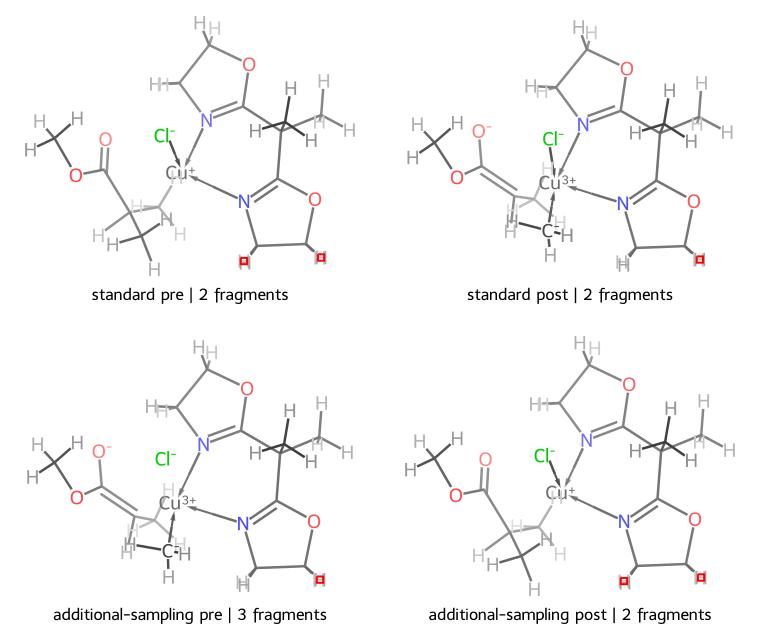
The top row contains the standard precursor and product; the bottom row contains the additional-sampling precursor and product. Each legend reports the fragment count. This pair is an additional representation and does not replace the standard endpoints.

Write the pair as XYZ (the default) or SDF files with save_pre_post_ts(...). SDF retains the reconstructed graph and the inferred three-dimensional conformer:

Python

pre_path, post_path = ts_frame.save_pre_post_ts("ts-endpoints", prefix="candidate")
sdf_pre_path, sdf_post_path = ts_frame.save_pre_post_ts(
    "ts-endpoints", prefix="candidate", format="sdf"
)
print(pre_path, post_path)

Endpoint file paths

Text Only

ts-endpoints/candidate_pre.xyz ts-endpoints/candidate_post.xyz

The files preserve the inferred three-dimensional candidate geometries. They are not optimized reactant and product structures.

When prefix is omitted, disk-backed frames include the source filename stem and frame ID in the generated names; memory-only frames fall back to ts_frame_<id>.

Call the same method on a parsed calculation file to export every TS frame. On a batch, each supported calculation file receives a separate directory named with its complete filename stem. Files without TS endpoint-export support are skipped with a warning. If source files in different directories have the same stem, MolOP adds a stable source-path digest to keep their output directories distinct:

Python

file_endpoints = trajectory.save_pre_post_ts("ts-endpoints", format="sdf")
batch_endpoints = ts_batch.save_pre_post_ts("ts-endpoints-batch", format="sdf", n_jobs=4)

Both mappings are keyed by original frame ID; the batch mapping adds the source path as its outer key.

Related operations

• Use filter_state("opt") and parsed_file.closest_optimized_frame for optimization trajectories.
• Use frame.vibrate(...) when a specific vibration, rather than the first one, is required.
• Export selected structures with Convert and export.